Activation Functions in Neural Networks: A Comprehensive Guide

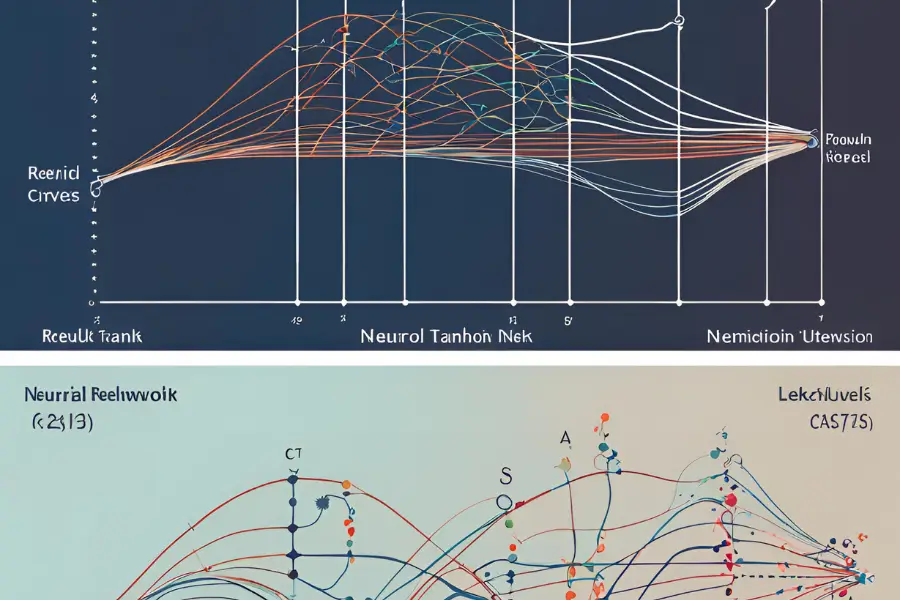
In the ever-evolving landscape of artificial intelligence, few components play as crucial a role as activation functions in neural networks. These mathematical operations are the spark that ignites the power of AI, enabling our models to capture the intricacies of the real world. As we embark on this exploration of activation functions, we’ll uncover their types, uses, and the profound impact they have on shaping modern machine learning algorithms.

Introduction to Activation Functions

At its core, an activation function is a mathematical operation applied to the output of a neuron in artificial neural networks. But why are these functions so essential? To understand their significance, we must first grasp the fundamental structure of neural networks.

Neural networks are composed of interconnected layers of artificial neurons, each processing and passing information to the next layer. Without activation functions, these networks would be limited to simple linear transformations, severely restricting their ability to learn complex patterns and relationships in data. In essence, activation functions introduce the critical element of non-linearity into the network.

Historically, the concept of activation functions has evolved significantly. In the early days of neural network research, simple step functions were used to mimic the “all-or-nothing” firing of biological neurons. However, as our understanding of machine learning deepened, more sophisticated non-linear functions emerged, dramatically enhancing the capabilities of neural networks.

Now that we’ve laid the groundwork, let’s delve deeper into the various types of activation functions and their unique characteristics.

Types of Activation Functions

Activation functions can be broadly categorized into two main types: linear and non-linear. Each type has its own set of properties and use cases, which we’ll explore in detail.

Linear Activation Functions

The simplest form of activation function is the linear function, defined as f(x) = x. While straightforward, linear activation functions have limited use in modern neural networks. Their primary drawback is their inability to solve non-linear problems, which constitute the majority of real-world scenarios.

Nevertheless, linear activation functions do have their place. They are occasionally used in the output layer of regression problems, where the goal is to predict a continuous value. However, for most intermediate layers and complex tasks, non-linear activation functions are the go-to choice.

Non-linear Activation Functions

Non-linear activation functions are the workhorses of modern neural networks. They allow networks to learn complex patterns and relationships in data. Let’s examine some of the most popular non-linear activation functions:

Sigmoid Function

The sigmoid function, also known as the logistic function, is one of the oldest and most well-known activation functions. It’s defined as:

σ(x) = 1 / (1 + e^(-x))

Key characteristics of the sigmoid function include:

• Outputs values between 0 and 1
• Smooth gradient, preventing “jumps” in output values
• Clear predictions in binary classification tasks

Despite its historical significance, the sigmoid function has fallen out of favor for hidden layers in deep networks due to the vanishing gradient problem. However, it still finds use in the output layer of binary classification problems and as gates in more complex architectures like Long Short-Term Memory (LSTM) networks.

Hyperbolic Tangent (tanh) Function

The tanh function is similar to the sigmoid but with a range of -1 to 1. Its formula is:

tanh(x) = (e^x – e^(-x)) / (e^x + e^(-x))

Compared to the sigmoid function, tanh has several advantages:

• Zero-centered output, which can help in centering the data for the next layer
• Steeper derivatives, which can lead to faster learning

While tanh generally performs better than sigmoid in hidden layers, it can still suffer from the vanishing gradient problem in very deep networks.

Rectified Linear Unit (ReLU)

ReLU has become one of the most popular activation functions in recent years. Its formula is deceptively simple:

f(x) = max(0, x)

Despite its simplicity, ReLU offers several significant benefits:

• Computational efficiency, as it’s a simple threshold operation
• Helps alleviate the vanishing gradient problem
• Induces sparsity in the network, which can be beneficial for feature learning

However, ReLU is not without its drawbacks. The “dying ReLU” problem occurs when neurons get stuck in a state where they always output zero, effectively becoming non-responsive to variations in input.

Leaky ReLU

To address the dying ReLU problem, variations like Leaky ReLU were introduced. Leaky ReLU is defined as:

f(x) = max(αx, x), where α is a small constant (usually 0.01)

This small modification allows a small, non-zero gradient when the unit is not active, which can help prevent neurons from getting stuck in a non-responsive state.

Softmax Function

The softmax function is a bit different from the others we’ve discussed. It’s typically used in the output layer of multi-class classification problems. Softmax converts a vector of real numbers into a probability distribution. Its formula for the i-th class is:

softmax(x_i) = e^(x_i) / Σ(e^(x_j))

Softmax ensures that the sum of probabilities across all classes equals 1, making it ideal for multi-class classification tasks.

Now that we’ve covered the main types of activation functions, let’s explore how they work in practice and their impact on neural network behavior.

How Activation Functions Work

To truly understand activation functions, we need to delve into their mathematical representations and visualize their behavior. Let’s break this down step by step.

Mathematical Representations

Each activation function has its own unique mathematical formula, as we’ve seen. These formulas determine how the function maps input values to output values. For instance, the sigmoid function squashes inputs into a range between 0 and 1, while ReLU simply returns the input if it’s positive, or zero otherwise.

Input and Output Ranges

The input and output ranges of activation functions play a crucial role in network behavior:

• Sigmoid and tanh have bounded outputs, which can help in stabilizing the network.
• ReLU and its variants have unbounded outputs for positive inputs, which can lead to faster learning in some cases.

Understanding these ranges is crucial when choosing an activation function for a specific task or layer in your network.

Effect on Neuron Activation

Activation functions determine when a neuron “fires” or activates. This behavior is analogous to biological neurons, which have a threshold for firing. In artificial neural networks:

• Sigmoid and tanh have smooth, continuous transitions.
• ReLU has a sharp transition at zero, mimicking a more binary on/off behavior.

This firing behavior influences how information flows through the network and how it learns patterns in the data.

Network Behavior

The choice of activation function can significantly impact overall network behavior:

• Non-linear functions allow the network to approximate complex functions and learn intricate patterns.
• The derivatives of activation functions play a crucial role in backpropagation, affecting how the network learns from errors.

To illustrate these concepts, let’s visualize the shapes and behaviors of different activation functions:

These visualizations help us understand how each function responds to different input values, which is crucial when choosing the right activation function for a specific task.

Choosing the Right Activation Function

Selecting the appropriate activation function is a critical decision that can significantly impact your neural network’s performance. Let’s explore the factors to consider and best practices for different scenarios.

Factors to Consider

When choosing an activation function, keep these key factors in mind:

• Problem type (e.g., binary classification, multi-class classification, regression)
• Network architecture (e.g., feedforward, CNN, RNN)
• Desired properties (e.g., differentiability, range, computational efficiency)
• Potential issues (e.g., vanishing gradients, dying neurons)

Best Practices for Different Architectures

Different neural network architectures often have different activation function requirements:

Convolutional Neural Networks (CNNs):

• ReLU and its variants are popular choices for hidden layers due to their computational efficiency and ability to mitigate the vanishing gradient problem.
• Softmax is typically used in the output layer for multi-class classification tasks.

Recurrent Neural Networks (RNNs) and Long Short-Term Memory (LSTM) networks:

• Tanh and sigmoid functions are often used in gates due to their bounded output ranges.
• ReLU can be used in simple RNNs but may lead to exploding gradients in some cases.

Feedforward networks:

• The choice varies based on the specific use case, but ReLU is often a good starting point for hidden layers.
• Output layer activation depends on the task (e.g., sigmoid for binary classification, linear for regression).

Impact on Model Performance

The choice of activation function can significantly affect various aspects of model performance:

• Training speed: ReLU and its variants often lead to faster training due to their computational simplicity and the reduced likelihood of vanishing gradients.
• Convergence: Some activation functions, like sigmoid and tanh, can slow down convergence in very deep networks due to saturation.
• Accuracy: The right activation function can lead to improved model accuracy by allowing the network to learn more complex patterns.

To illustrate these points, consider the following example:

This graph demonstrates how different activation functions can affect the learning process and final performance of a neural network on a specific task.

Implementation and Practical Considerations

Now that we understand the theory behind activation functions, let’s explore how to implement them in practice and some key considerations for optimizing your neural networks.

Python Implementations

Here’s a quick look at how you can implement some common activation functions in Python:

import numpy as np

def sigmoid(x):
    return 1 / (1 + np.exp(-x))

def tanh(x):
    return np.tanh(x)

def relu(x):
    return np.maximum(0, x)

def leaky_relu(x, alpha=0.01):
    return np.where(x > 0, x, alpha * x)

def elu(x, alpha=1.0):
    return np.where(x > 0, x, alpha * (np.exp(x) - 1))

def softmax(x):
    exp_x = np.exp(x - np.max(x, axis=-1, keepdims=True))
    return exp_x / np.sum(exp_x, axis=-1, keepdims=True)

# Usage example
x = np.array([-2, -1, 0, 1, 2])
print("Input:", x)
print("ReLU:", relu(x))
print("Leaky ReLU:", leaky_relu(x))
print("ELU:", elu(x))
print("Sigmoid:", sigmoid(x))
print("Tanh:", tanh(x))
print("Softmax:", softmax(x))
        

import tensorflow as tf

def tensorflow_example():
    model = tf.keras.Sequential([
        tf.keras.layers.Dense(64, activation='relu', input_shape=(784,)),
        tf.keras.layers.Dense(32, activation='relu'),
        tf.keras.layers.Dense(10, activation='softmax')
    ])
    
    # Custom activation function
    def custom_activation(x):
        return tf.nn.relu(x) * tf.sigmoid(x)
    
    custom_layer = tf.keras.layers.Dense(32, activation=custom_activation)

    return model

# Usage
tf_model = tensorflow_example()
print("TensorFlow model summary:")
tf_model.summary()
        

Debugging and Optimization

When working with activation functions, keep these tips in mind:

• Monitor for vanishing or exploding gradients, especially in deep networks.
• Use techniques like batch normalization to help stabilize the network.
• Experiment with different activation functions and compare performance.
• Consider using adaptive learning rates to help overcome challenges with certain activation functions.

Future Trends

The field of activation functions is continuously evolving. Some exciting areas of research include:

• Adaptive activation functions that adjust during training.
• Novel activation functions designed for specific tasks or architectures.
• Activation functions inspired by biological neural networks.

As we conclude our comprehensive guide to activation functions, it’s clear that these mathematical operations are far more than mere technicalities. They are the lifeblood of neural networks, enabling our models to capture the complexities of the real world.

From the sigmoid’s smooth transitions to ReLU’s computational efficiency, each activation function offers unique strengths that, when applied judiciously, can dramatically enhance a neural network’s capabilities. As the field of AI continues to evolve, so too will our understanding and application of activation functions.

By mastering these fundamental building blocks, you’re not just optimizing algorithms – you’re shaping the future of intelligent systems. The next breakthrough in AI might just come from a novel activation function, and armed with the knowledge from this guide, you’re well-equipped to be at the forefront of that innovation.

Remember, the journey of mastering activation functions is ongoing. Continual experimentation, staying updated with the latest research, and understanding the nuances of different functions will be key to your success in the exciting world of neural networks and artificial intelligence.